Matplotlib Contour Plots - A Complete Reference

In this article, we will be learning about how to create contour plots in Python using the contour function and Matpotlib. We will be looking at the different types of plotting functions and the different types of plots that are created through them. We will also be looking at the code along with a detailed explanation of how to go along with it.

What are contour plots?

Contours are a 2-Dimensional representation of a 3-D surface, with curves and joints. It is plotted by using a contour function(Z) which is a function of two variables(X, Y).

For working with contour plots, we need two libraries – Matplotlib and NumPy. Let’s install them.

Matplotlib is a Python-based Plotting library used to create charts and plots. To install Matplotlib, type the command:

pip install matplotlib

We will be needing another library – Python Numpy to create our contour plots. To install it, type the command:

pip install numpy

Creating a Contour Plot

With the basic requirements in place, let’s get started with plotting our contour plots right away.

Importing the important libraries:

import matplotlib.pyplot as plt
import numpy as nump

Initialising the X, Y variables

The variables X and Y get initialized in the code below with the 3-Dimensional coordinates for the plot.

element_ofx = nump.arange(0, 25, 4)
element_ofy = nump.arange(0, 26, 4)

Creating the contour function Z with the two variables

[grid_ofX, grid_ofY] = nump.meshgrid(element_ofx, element_ofy)

fig, holowplt= plt.subplots(1, 1)

grid_ofZ = nump.cos(grid_ofX / 1) - nump.sin(grid_ofY / 2)

Plotting the contour chart

holowplt.contour(grid_ofX, grid_ofY, grid_ofZ)

holowplt.set_title('Contour Plot')
holowplt.set_xlabel('features of x-axis')
holowplt.set_ylabel('features of y-axis')

plt.show()

The code below demonstrates how simple, hollow matplotlib contour plots are created:

import matplotlib.pyplot as plt
import numpy as nump

element_ofx = nump.arange(0, 25, 4)
element_ofy = nump.arange(0, 26, 4)

# This numpy function creates 2-dimensional grid
[grid_ofX, grid_ofY] = nump.meshgrid(element_ofx, element_ofy)

# plots 2 graphs in one chart
fig, holowplt = plt.subplots(1, 1)

# Mathematical function for contour
grid_ofZ = nump.cos(grid_ofX / 1) - nump.sin(grid_ofY / 2)

# plots contour lines
holowplt.contour(grid_ofX, grid_ofY, grid_ofZ)

holowplt.set_title('Contour Plot')
holowplt.set_xlabel('features of x-axis')
holowplt.set_ylabel('features of y-axis')

plt.show()

Output:

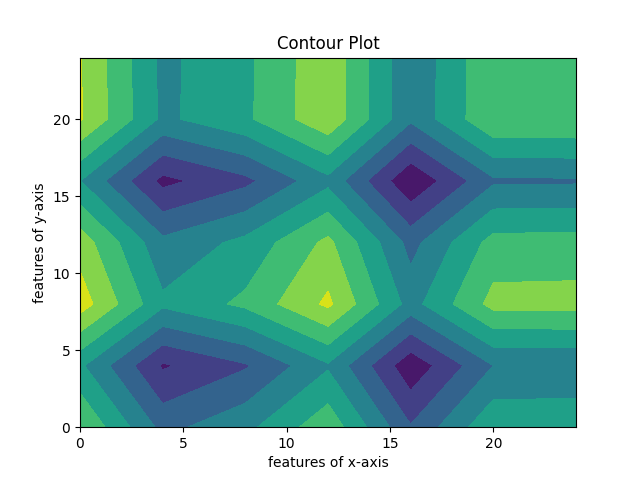
Filled Contour Plots

In this example, we will be creating filled contour plots instead of hollow ones. To create filled plots, we will be using ‘contourf’ function. The whole program is very similar to the previous example with some slight changes.

Plotting the contour chart

fillplot.contourf(grid_ofX, grid_ofY, grid_ofZ)

fillplot.set_title('Contour Plot')
fillplot.set_xlabel('features of x-axis')
fillplot.set_ylabel('features of y-axis')

Let’s look at the whole code, to get a better understanding:

import matplotlib.pyplot as plt
import numpy as nump

element_ofx = nump.arange(0, 25, 4)
element_ofy = nump.arange(0, 26, 4)

# This numpy function creates 2-dimensional grid
[grid_ofX, grid_ofY] = nump.meshgrid(element_ofx, element_ofy)

# plots 2 graphs in one chart
fig, fillplot = plt.subplots(1, 1)

# Mathematical function for contour
grid_ofZ = nump.cos(grid_ofX / 1) - nump.sin(grid_ofY / 2)

# plots contour lines
fillplot.contourf(grid_ofX, grid_ofY, grid_ofZ)

fillplot.set_title('Contour Plot')
fillplot.set_xlabel('features of x-axis')
fillplot.set_ylabel('features of y-axis')

plt.show()

Output:

Using state-based interface for contour plot

Matplotlib sub-module allows us to plot contours with varied interfaces. In this section, we will be looking at matplotlib modes that plot contours in a way that resembles the MATLAB interface.

Let’s understand code by code, how to plot a contour using this submodule.

Importing libraries

In this particular example, we will be mainly using two libraries, similar to the previous examples – Matplotlib and Numpy.

import numpy as np
import matplotlib.pyplot as plt

Initialisation of variables

delta = 0.18
element_ofx = np.arange(1.8, 2.8, delta)
element_ofy = np.arange(1.5, 3.6, delta)
grid_ofX, grid_ofY = np.meshgrid(element_ofx, element_ofy)
grid_ofZ = (np.exp(grid_ofX + grid_ofY))

Let’s look at the complete code to get a better understanding:

# Importing libraries
import numpy as np
import matplotlib.pyplot as plt

# variable initialisation
delta = 0.18
element_ofx = np.arange(1.8, 2.8, delta)
element_ofy = np.arange(1.5, 3.6, delta)
grid_ofX, grid_ofY = np.meshgrid(element_ofx, element_ofy)
grid_ofZ = (np.exp(grid_ofX + grid_ofY))

# Contour plotting
plot = plt.contour(grid_ofX, grid_ofY, grid_ofZ)

grid_format = {}
numscale = ['1', '2', '3', '4', '5', '6', '7']
for lvls, s in zip(plot.levels, numscale):
	grid_format[lvls] = s
plt.clabel(plot, plot.levels, inline = True,
		fmt = grid_format, fontsize = 10)

plt.title('Contour in Matlab interface')
plt.show()

Conclusion

This article is a good foundation for your Matplotlib learning. All the topics and concepts are put forward in an easy-to-understand method so that readers can easily grab on all the basics. A good overview of the whole article will help you to easily venture further ahead with more advanced Matplotlib concepts.