🚀 Supercharge your YouTube channel's growth with AI.
Try YTGrowAI FreeProbability Distributions with Python (Implemented Examples)

Probability Distributions are mathematical functions that describe all the possible values and likelihoods that a random variable can take within a given range.
Probability distributions help model random phenomena, enabling us to obtain estimates of the probability that a certain event may occur.
In this article, we’ll implement and visualize some of the commonly used probability distributions using Python
Common Probability Distributions
The most common probability distributions are as follows:
- Uniform Distribution
- Binomial Distribution
- Poisson Distribution
- Exponential Distribution
- Normal Distribution
Let’s implement each one using Python.
1. Uniform Distributions
The uniform distribution defines an equal probability over a given range of continuous values. In other words, it is a distribution that has a constant probability.
The probability density function for a continuous uniform distribution on the interval [a,b] is:

Example – When a 6-sided die is thrown, each side has a 1/6 chance.
Implementing and visualizing uniform probability distribution in Python using scipy module.
#Importing required libraries
from scipy.stats import uniform
import seaborn as sb
import matplotlib.pyplot as plt
import numpy as np

#taking random variables from Uniform distribution
data = uniform.rvs(size = 100000, loc = 5, scale=10)

#Plotting the results
sb.set_style('whitegrid')
ax = sb.distplot(data, bins = 30, color = 'k')
ax.set(xlabel = 'interval')
plt.show()
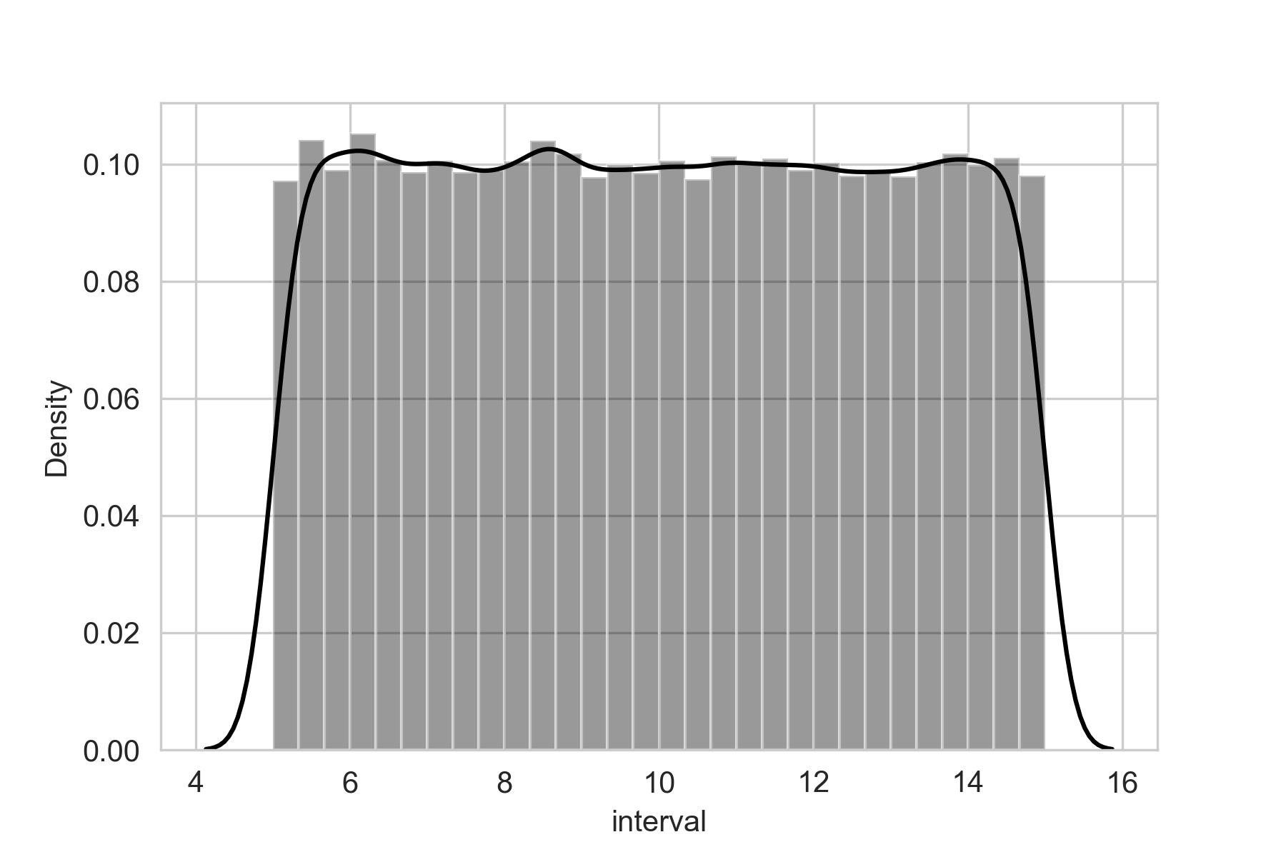
scipy.stats module has a uniform class in which the first argument is the lower bound and the second argument is the range of the distribution.
loc– lower bound.scale– range of distribution.
For example, if we want to randomly pick values from a uniform distribution in the range of 5 to 15. Then loc parameter will 5 as it is the lower bound. scale parameter will be set to 10 as if we add loc and scale we will get 15 as the upper bound.
2. Binomial Distribution
The Binomial distribution is the discrete probability distribution. it has parameters n and p, where p is the probability of success, and n is the number of trials.
Suppose we have an experiment that has an outcome of either success or failure:
- we have the probability p of success
- then Binomial pmf can tell us about the probability of observing k
- if the experiment is performed n number of times.
Probability mass function of a Binomial distribution is:

#Importing required modules
import seaborn as sb
import matplotlib.pyplot as plt
import numpy as np
from scipy.stats import binom

#Applying the binom class
pb = binom(n = 20, p = 0.6)

x = np.arange(1,21)
pmf = pb.pmf(x)

#Visualizing the distribution
sb.set_style('whitegrid')
plt.vlines(x ,0, pb.pmf(x), colors='k', linestyles='-', lw=5)
plt.ylabel('Probability')
plt.xlabel('Intervals')
plt.show()

scipy.stats module has binom class which needs following input parametes:
- n = number of intervals
- p = probability of success
The binom class has .pmf method which requires interval array as an input argument, the output result is the probability of the corresponding values.
BERNOULLI Distribution
It is a special case of the binomial distribution for n = 1. In other words, it is a binomial distribution with a single trial.
The probability mass function of Bernoulli distribution is given by:

#Importing the required modules
import seaborn as sb
import matplotlib.pyplot as plt
import numpy as np
from scipy.stats import bernoulli

#Applying the bernoulli class
data = bernoulli.rvs(size = 1000 , p = 0.8)

#Visualizing the results
sb.set_style('whitegrid')
sb.displot(data, discrete=True, shrink=.8 , color = 'k')
plt.show()

We need to specify the probability p as the input parameter to the bernoulli class object. To pick random values from the distribution the Bernoulli class has .rvs method which takes an optional size parameter(number of samples to pick).
3. Poisson Distribution
It gives us the probability of a given number of events happening in a fixed interval of time if these events occur with a known constant mean rate and independently of each other.
The mean rate is also called as Lambda (λ).
Suppose we own a fruit shop and on an average 3 customers arrive in the shop every 10 minutes. The mean rate here is 3 or λ = 3. Poisson probability distributions can help us answer questions like what is the probability that 5 customers will arrive in the next 10 mins?
The probability mass function is given by:

#Importing the required modules
import seaborn as sb
import matplotlib.pyplot as plt
import numpy as np
from scipy.stats import poisson

#Applying the poisson class methods
x = np.arange(0,10)
pmf = poisson.pmf(x,3)

#Visualizing the results
sb.set_style('whitegrid')
plt.vlines(x ,0, pmf, colors='k', linestyles='-', lw=6)
plt.ylabel('Probability')
plt.xlabel('intervals')
plt.show()

The poisson class from scipy.stats module has only one shape parameter: mu which is also known as rate as seen in the above formula. .pmf will return the probability values of the corresponding input array values.
4. Exponential Distribution
In probability and statistics, the exponential distribution is the probability distribution of the time between events in a Poisson point process. The exponential distribution describes the time for a continuous process to change state.
Poisson distribution deals with the number of occurrences of an event in a given period and exponential distribution deals with the time between these events.
The exponential distribution may be viewed as a continuous counterpart of the geometric distribution.

Here λ > 0 is the parameter of the distribution, often called the rate parameter.
#Importing required modules
import seaborn as sb
import matplotlib.pyplot as plt
import numpy as np
from scipy.stats import expon

#Applying the expon class methods
x = np.linspace(0.001,10, 100)
pdf = expon.pdf(x)

#Visualizing the results
sb.set_style('whitegrid')
plt.plot(x, pdf , 'r-', lw=2, alpha=0.6, label='expon pdf' , color = 'k')
plt.xlabel('intervals')
plt.ylabel('Probability Density')
plt.show()

Input parameters to expon class from scipy.stats module are as follows:
x: quantilesloc: [optional] location parameter. Default = 0scale: [optional] scale parameter. Default = 1
To calculate probability density of the given intervals we use .pdf method.
5. Normal Distribution
A Normal Distribution is also known as a Gaussian distribution or famously Bell Curve.
The probability density function (pdf) for Normal Distribution:

where, μ = Mean , σ = Standard deviation , x = input value.
# import required libraries
from scipy.stats import norm
import numpy as np
import matplotlib.pyplot as plt
import seaborn as sb

# Creating the distribution
data = np.arange(1,10,0.01)
pdf = norm.pdf(data , loc = 5.3 , scale = 1 )

#Visualizing the distribution

sb.set_style('whitegrid')
sb.lineplot(data, pdf , color = 'black')
plt.ylabel('Probability Density')

scipy.stats module has norm class for implementation of normal distribution.
The location loc keyword specifies the mean. The scale scale keyword specifies the standard deviation in the above code.
to calculate the probability density in the given interval we use .pdf method providing the loc and scale arguments.
Conclusion
In this article, we implemented a few very commonly used probability distributions using scipy.stats module. we also got an intuition on what the shape of different distributions looks like when plotted.
Happy Learning!


