🚀 Supercharge your YouTube channel's growth with AI.
Try YTGrowAI FreeNormal Distribution in Python

Even if you are not in the field of statistics, you must have come across the term “Normal Distribution”.
A probability distribution is a statistical function that describes the likelihood of obtaining the possible values that a random variable can take. By this, we mean the range of values that a parameter can take when we randomly pick up values from it.
A probability distribution can be discrete or continuous.
Suppose in a city we have heights of adults between the age group of 20-30 years ranging from 4.5 ft. to 7 ft.
If we were asked to pick up 1 adult randomly and asked what his/her (assuming gender does not affect height) height would be? There’s no way to know what the height will be. But if we have the distribution of heights of adults in the city, we can bet on the most probable outcome.
What is Normal Distribution?
A Normal Distribution is also known as a Gaussian distribution or famously Bell Curve. People use both words interchangeably, but it means the same thing. It is a continuous probability distribution.
The probability density function (pdf) for Normal Distribution:

where, μ = Mean , σ = Standard deviation , x = input value.
Terminology:
- Mean – The mean is the usual average. The sum of total points divided by the total number of points.
- Standard Deviation – Standard deviation tells us how “spread out” the data is. It is a measure of how far each observed value is from the mean.
Looks daunting, isn’t it? But it is very simple.
1. Example Implementation of Normal Distribution
Let’s have a look at the code below. We’ll use numpy and matplotlib for this demonstration:
# Importing required libraries

import numpy as np
import matplotlib.pyplot as plt

# Creating a series of data of in range of 1-50.
x = np.linspace(1,50,200)

#Creating a Function.
def normal_dist(x , mean , sd):
    prob_density = (np.pi*sd) * np.exp(-0.5*((x-mean)/sd)**2)
    return prob_density

#Calculate mean and Standard deviation.
mean = np.mean(x)
sd = np.std(x)

#Apply function to the data.
pdf = normal_dist(x,mean,sd)

#Plotting the Results
plt.plot(x,pdf , color = 'red')
plt.xlabel('Data points')
plt.ylabel('Probability Density')

2. Properties of Normal Distribution
The normal distribution density function simply accepts a data point along with a mean value and a standard deviation and throws a value which we call probability density.
We can alter the shape of the bell curve by changing the mean and standard deviation.
Changing the mean will shift the curve towards that mean value, this means we can change the position of the curve by altering the mean value while the shape of the curve remains intact.
The shape of the curve can be controlled by the value of Standard deviation. A smaller standard deviation will result in a closely bounded curve while a high value will result in a more spread out curve.
Some excellent properties of a normal distribution:
- The mean, mode, and median are all equal.
- The total area under the curve is equal to 1.
- The curve is symmetric around the mean.
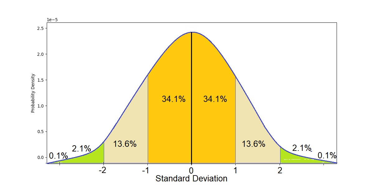
Empirical rule tells us that:
- 68% of the data falls within one standard deviation of the mean.
- 95% of the data falls within two standard deviations of the mean.
- 99.7% of the data falls within three standard deviations of the mean.
It is by far one of the most important distributions in all of the Statistics. The normal distribution is magical because most of the naturally occurring phenomenon follows a normal distribution. For example, blood pressure, IQ scores, heights follow the normal distribution.
Calculating Probabilities with Normal Distribution
To find the probability of a value occurring within a range in a normal distribution, we just need to find the area under the curve in that range. i.e. we need to integrate the density function.
Since the normal distribution is a continuous distribution, the area under the curve represents the probabilities.
Before getting into details first let’s just know what a Standard Normal Distribution is.
A standard normal distribution is just similar to a normal distribution with mean = 0 and standard deviation = 1.
Z = (x-μ)/ σ
The z value above is also known as a z-score. A z-score gives you an idea of how far from the mean a data point is.
If we intend to calculate the probabilities manually we will need to lookup our z-value in a z-table to see the cumulative percentage value. Python provides us with modules to do this work for us. Let’s get into it.
1. Creating the Normal Curve
We’ll use scipy.norm class function to calculate probabilities from the normal distribution.
Suppose we have data of the heights of adults in a town and the data follows a normal distribution, we have a sufficient sample size with mean equals 5.3 and the standard deviation is 1.
This information is sufficient to make a normal curve.
# import required libraries
from scipy.stats import norm
import numpy as np
import matplotlib.pyplot as plt
import seaborn as sb

# Creating the distribution
data = np.arange(1,10,0.01)
pdf = norm.pdf(data , loc = 5.3 , scale = 1 )

#Visualizing the distribution

sb.set_style('whitegrid')
sb.lineplot(data, pdf , color = 'black')
plt.xlabel('Heights')
plt.ylabel('Probability Density')
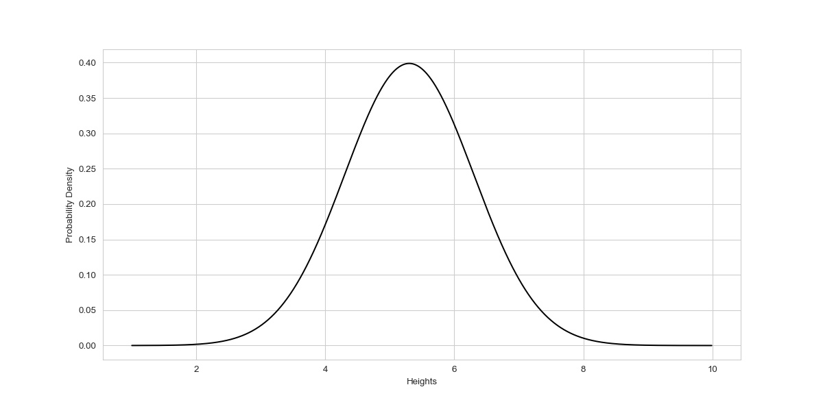
The norm.pdf( ) class method requires loc and scale along with the data as an input argument and gives the probability density value. loc is nothing but the mean and the scale is the standard deviation of data. the code is similar to what we created in the prior section but much shorter.
2. Calculating Probability of Specific Data Occurance
Now, if we were asked to pick one person randomly from this distribution, then what is the probability that the height of the person will be smaller than 4.5 ft. ?

The area under the curve as shown in the figure above will be the probability that the height of the person will be smaller than 4.5 ft if chosen randomly from the distribution. Let’s see how we can calculate this in python.
The area under the curve is nothing but just the Integration of the density function with limits equals -∞ to 4.5.
norm(loc = 5.3 , scale = 1).cdf(4.5)
0.211855 or 21.185 %
The single line of code above finds the probability that there is a 21.18% chance that if a person is chosen randomly from the normal distribution with a mean of 5.3 and a standard deviation of 1, then the height of the person will be below 4.5 ft.
We initialize the object of class norm with mean and standard deviation, then using .cdf( ) method passing a value up to which we need to find the cumulative probability value. The cumulative distribution function (CDF) calculates the cumulative probability for a given x-value.
Cumulative probability value from -∞ to ∞ will be equal to 1.
Now, again we were asked to pick one person randomly from this distribution, then what is the probability that the height of the person will be between 6.5 and 4.5 ft. ?

cdf_upper_limit = norm(loc = 5.3 , scale = 1).cdf(6.5)
cdf_lower_limit = norm(loc = 5.3 , scale = 1).cdf(4.5)

prob = cdf_upper_limit - cdf_lower_limit
print(prob)
0.673074 or 67.30 %
The above code first calculated the cumulative probability value from -∞ to 6.5 and then the cumulative probability value from -∞ to 4.5. if we subtract cdf of 4.5 from cdf of 6.5 the result we get is the area under the curve between the limits 6.5 and 4.5.
Now, what if we were asked about the probability that the height of a person chosen randomly will be above 6.5ft?
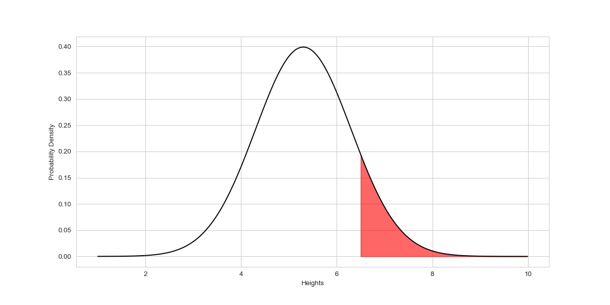
It’s simple, as we know the total area under the curve equals 1, and if we calculate the cumulative probability value from -∞ to 6.5 and subtract it from 1, the result will be the probability that the height of a person chosen randomly will be above 6.5ft.
cdf_value = norm(loc = 5.3 , scale = 1).cdf(6.5)
prob = 1- cdf_value
print(prob)
0.115069 or 11.50 %.
That’s a lot to sink in, but I encourage all to keep practicing this essential concept along with the implementation using python.
The complete code from above implementation:
# import required libraries
from scipy.stats import norm
import numpy as np
import matplotlib.pyplot as plt
import seaborn as sb

# Creating the distribution
data = np.arange(1,10,0.01)
pdf = norm.pdf(data , loc = 5.3 , scale = 1 )

#Probability of height to be under 4.5 ft.
prob_1 = norm(loc = 5.3 , scale = 1).cdf(4.5)
print(prob_1)

#probability that the height of the person will be between 6.5 and 4.5 ft.

cdf_upper_limit = norm(loc = 5.3 , scale = 1).cdf(6.5)
cdf_lower_limit = norm(loc = 5.3 , scale = 1).cdf(4.5)

prob_2 = cdf_upper_limit - cdf_lower_limit
print(prob_2)

#probability that the height of a person chosen randomly will be above 6.5ft

cdf_value = norm(loc = 5.3 , scale = 1).cdf(6.5)
prob_3 = 1- cdf_value
print(prob_3)
Conclusion
In this article, we got some idea about Normal Distribution, what a normal Curve looks like, and most importantly its implementation in Python.
Happy Learning !