🚀 Supercharge your YouTube channel's growth with AI.
Try YTGrowAI FreeRuntime Complexities of Data Structures in Python

In this article, we will be looking at the different types of runtime complexities associated with programming algorithms. We will be looking at time and space complexities, different case scenarios, and specific time complexities. We will also be looking up at time complexities of different python operations.
What is meant by runtime complexities in programming?
When applying an algorithm, each data structure executes a variety of actions. Operations like iterating through a group of elements, adding an item at a certain position in the group, removing, updating, or generating a clone of an element or the whole group. These actions are just a few of the essential and general operations. All types of data structures that we use in programming have a significant impact on the application’s performance. This is caused because data structure operating processes have varied time and space complexities.
1. Complexity of Space
The term “space complexity” states to the quantity of size or memory space an algorithm can take up. It comprises auxiliary space, as well as space, which is taken by data provided as input.
The additional space or impermanent space that an algorithm requires is denoted as auxiliary space.
The overall space consumed by an algorithm regarding the size of the input is known as its complexity of space.
2. Complexity of Time
When the operations take up time which when measured to know how long it takes to accomplish the desirable process, then it is denoted as the complexity of time. It is usually denoted as ‘O’ or the Big-O symbolization, which is employed to quantify time complexity. The means of computing the competence of a process reliant on how big the input is known as ‘O’ or Big-O notation.
The means of calculating the efficiency of an operation depending on the size of the input is known as Big-O notation.
Types:
Here we will be going through the different types of runtime complexities:
Constant time or O(1)
The first complexity we will look up is this one. At a point where the algorithm is taking up time which is independent of the input elements, then the algorithm is denoted an O(1) or constant time (n).
Here the measure of how much time it takes to complete an action is consistent irrespective of the magnitude of your input collection. This implies that regardless of the number of input components dealt with, the operating procedures of the algorithm will continually take an equal quantity of time. For instance, reading the first member of a series is constantly O(1), irrespective of how vast the series is.
Logarithmic time or O(log n)
The second complexity we will be looking up is this type of process where the data provided as the input gets reduced with each passing individual stage of the procedure, the algorithm talked about here has logarithmic time complexity. Generally, O(log n) procedures involve algorithms like binary trees and binary search.
Linear time or O(n)
The third process we will be assessing is when there is a straight and linear relationship between the elapsed time by the algorithm and the magnitude of the quantity of data provided as input, then it has linear time complexity. Here in this particular scenario, the algorithm requires to evaluate all of the objects in the input data, making this the top suitable time complexity.
Quasilinear time or (n log n)
In this case, too, input elements have logarithmic time complexity but individual processes are split into several parts. Sorting operations like Merge sorts, tim sort, or heap sort are a few instances of optimal sorting algorithms.
The data provided as input is divided into many sub-lists until single elements are left in each sub-list, and then those sub-lists are amalgamated into an organized list. As a result, the time complexity is O (nlogn).
Quadratic time or O(n^2)
The fifth and sixth processes are similar in nature but very different in magnitude. Time taken here to operate is comparative to the square of the data provided as input present in the group, thus time complexity for this process is quadratic. When the algorithm necessitates executing a linear time operation on input data’s every element, the time complexity gets reliant on the squares of the elements. For instance, O(n2) takes place in bubble sort.
Exponential time or O(2^n)
When the expansion of an algorithm doubles with every addition to the input data set, it is said to have an exponential time complexity. In the sixth process, the expansion of an algorithm doubles with every accumulation to the group of input data, and its time complexity is denoted as exponential. Brute-force methods are known for having this level of time complexity. For instance, we can find O(2 n) time complexity in the recursive calculation of Fibonacci numbers.
Factorial time (n!)
The last process we will be looking up to, talks about the time it takes to calculate each variation possible in an operation, which is factorial of the size of the objects in the input collection, thus the procedure is denoted an (n!) complexity.
As an example, Heap’s algorithm computes all likely variations of n number of objects. All the algorithms are very slow in performance which has O(n!) time complexity.

Types of case in data structure’s time complexities:
Best case scenario: Best case scenario: We determine the lower lap on an algorithm’s execution time in the best-case study. When the data structures and objects in the group, furthermore to the parameters, are at their best levels, the best-case scenario happens. As a result, only small-scale operations are carried out. In a linear search, e.g., scenario, where the best case is likely, is when x (the object searched) is present at the top of the list. In the best-case scenario, the number of actions remains unchanged (not reliant on the number of input elements). So, in this scenario, it has O(1) time complexity.
Average case scenario: This happens when we describe complexity as reliant on the data provided as input and how uniformly it has been distributed. We consider all potential inputs and compute the time it will take to calculate all of them in average-case analysis. To find out, simply divide the number of inputs by the added product of all computed values.
Worst-case scenario: Processes that involve locating an item that is located as the final item in a big-sized group, for example, a list, with the algorithm iterating throughout the group from the first item. For example, when x is not present in the list, an algorithm like linear search in that the iteration compares x to all of the entries. This would result in an O(n) run-time.
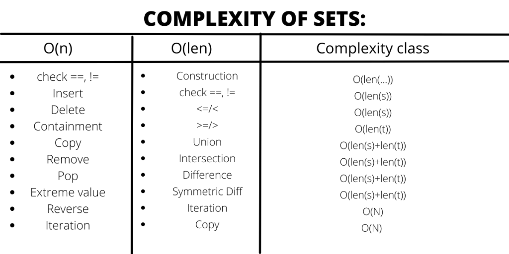
Time complexities of different data structures in python:


Conclusion
It is hoped that this article helped you to understand the different time complexities and which python data structure takes up what time complexity. After understanding the basic concepts of complexities, now you can find time complexities of data structures and observe the complexities in a sequence of operations.


