🚀 Supercharge your YouTube channel's growth with AI.
Try YTGrowAI FreeSciPy Find Peaks: Detect Signal Maxima


A sampled signal can have small fluctuations alongside the peaks you want to keep. SciPy’s find_peaks locates local maxima in a one-dimensional signal and can filter them with conditions such as height or distance.
I’ll show how to use find_peaks to select peaks with conditions that fit your signal, then measure their widths.
TL;DR: Find Peaks with SciPy
Use scipy.signal.find_peaks on a one-dimensional array to get the sample indices of local maxima, then add conditions such as prominence or distance to keep the peaks that fit your signal.
- Import with from scipy.signal import find_peaks.
- Choose height for absolute amplitude and prominence for separation from the local contour.
- Returned indices count samples, not seconds. convert them using your sampling interval.
What Does scipy.signal.find_peaks Return?
For a one-dimensional input, scipy.signal.find_peaks returns local-maximum indices and a dictionary of calculated peak properties.
find_peaks accepts one one-dimensional signal at a time. A multichannel recording needs a separate call per channel, with the channel label kept beside returned indices.
How to Find and Measure Peaks Step by Step
I ran the source with SciPy 1.18.1 and NumPy 2.5.4. Its short fixed array makes the selected positions directly checkable against input values.
Step 1: Import find_peaks and prepare a signal
The function import comes from scipy.signal. The signal here contains three candidate maxima. Its values are listed in the named source file.
import numpy as np
import scipy
from scipy.signal import find_peaks, peak_widths

# The selected peaks are at indices 3, 6 and 10.
signal = np.array([0, 1, 0, 2, 0, 1, 4, 1, 0, 0, 3, 0, 0], dtype=float)
peaks, properties = find_peaks(signal, prominence=1.5, distance=3, width=(None, None))
widths, width_heights, left_ips, right_ips = peak_widths(signal, peaks, rel_height=0.5)
print(f"SciPy {scipy.__version__}")
print("peak indices:", peaks.tolist())
print("peak heights:", signal[peaks].tolist())
print("prominences:", properties["prominences"].tolist())
print("widths at half prominence (samples):", np.round(widths, 2).tolist())
print("half-prominence heights:", np.round(width_heights, 2).tolist())
Run the complete source file with .venv/bin/python find_peaks_demo.py. The output below is the captured result of that command.
SciPy 1.18.1
peak indices: [3, 6, 10]
peak heights: [2.0, 4.0, 3.0]
prominences: [2.0, 4.0, 3.0]
widths at half prominence (samples): [1.0, 1.33, 1.0]
half-prominence heights: [1.0, 2.0, 1.5]
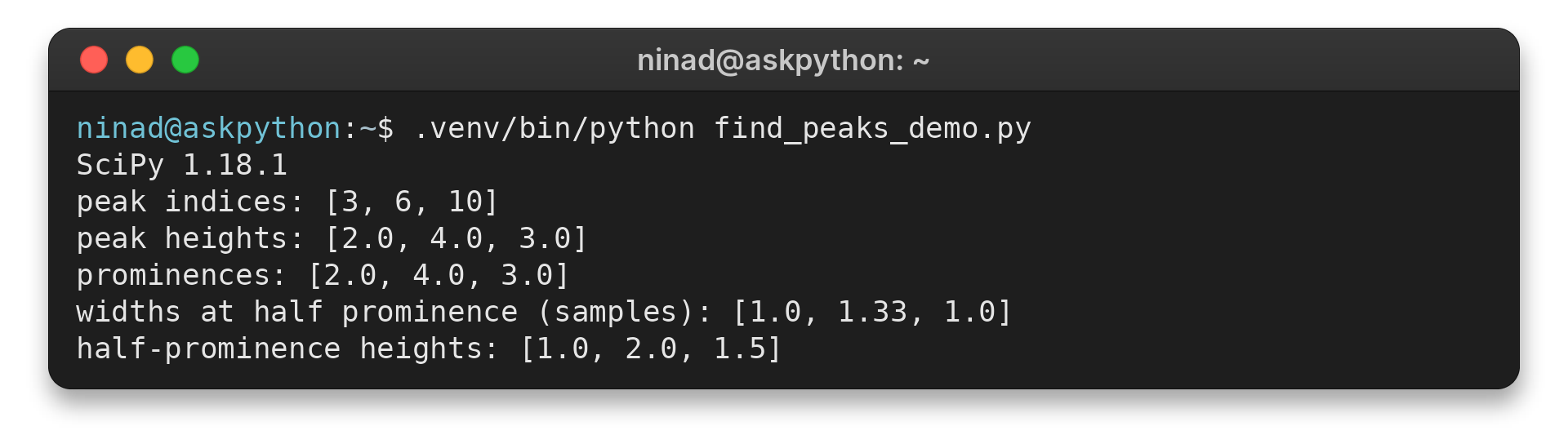
The output shows that the peak at index 6 has the largest value and prominence in this array.
For an amplitude window, pass height=(1, 4). The lower and upper endpoints are included.
Step 2: Choose conditions that match the signal
Threshold measures the vertical difference between a candidate and its immediate neighbors, so a broad summit can pass height while failing threshold. Use prominence when separation from the surrounding contour matters more than the immediate rise, and choose the criterion that fits the measurement task.
| Condition | What it measures | Choose it when |
|---|---|---|
| height | Peak’s absolute sample value | A fixed amplitude floor or ceiling matters |
| threshold | Vertical difference from the immediate neighbors | You need a sharp local rise and fall |
| prominence | Peak’s height above its local contour line | Baseline varies and local separation matters |
| distance | Minimum horizontal separation in samples | Nearby detections should collapse to one candidate |
| width | Width at a relative prominence height, in samples | Broad and narrow events have different meanings |
| plateau_size | Flat-top length in samples | Flat peaks should be selected by their span |
Step 3: Read the properties and measure width
With rel_height=0.5, peak_widths reports width halfway down a peak’s prominence contour, which equals conventional FWHM only when that contour matches the chosen baseline.
In evenly sampled data, multiply width and fractional crossing positions by the sampling interval to express them in time. A zero relative height can produce a zero-width warning. The left_ips and right_ips values mark the fractional positions where that width begins and ends.
Step 4: Validate candidates against the measurement
Use a small selection of known input segments to confirm which candidates the current settings keep. A candidate close to the bound is more revealing than another clear example because it tests the decision boundary.
Which find_peaks Edge Cases Should You Check?
NaN values can produce unexpected results, so inspect the input before detection. Use np.isnan(signal).any() to locate them and process contiguous valid samples when replacement is not supported by the measurement model.
| Case | Effect | Response |
|---|---|---|
| NaN values | Detection may be unexpected near missing samples | Remove or replace NaNs using a domain-appropriate method before detection |
| Flat-topped peak | Middle sample represents the local maximum | Use plateau_size to filter by flat-top span |
| Peak at first or last sample | No two-sided neighbor comparison is available | Handle boundary events explicitly if they matter |
| Negative-going trough | It is a local minimum and needs a separate transformation | Run detection on the negated signal, then map indices to the original data |
| Irregular timestamps | Duration depends on timestamp spacing | Resample first or apply time-based spacing after detection |
A flat-topped peak has repeated adjacent samples at the same maximum value. SciPy returns the midpoint and, when plateau_size is requested, reports the span and left_edges/right_edges for its limits. Compare those edge positions when the application cares about the full plateau rather than its midpoint alone.
To detect troughs, apply find_peaks to the negated signal and use the resulting indices to read the original values. Negation changes the amplitude sign but preserves each sample’s position, so the indices remain aligned with the source array.
The first and last samples cannot meet the two-neighbor local-maximum test because one side is missing from the array. If an event can touch an endpoint, apply a separate boundary rule or include surrounding samples from the recording before detection.
With irregular timestamps, equal sample distances can represent unequal elapsed times, and distance counts positions rather than enforcing a fixed duration. Use stored timestamps to compare elapsed spacing after detection. Resample only if interpolation is valid for the analysis, then keep the new sampling interval with sample-based bounds.
Filtering can move a maximum or broaden a feature, so compare detections before and after preprocessing. The scipy.signal filtering guide explains that as a separate choice.
Choosing the Right Parameters
Convert a time interval to a sample count before using it as distance.
- At 100 samples per second, an interval of 0.2 seconds maps to 20 samples.
Use ceil(T / dt) so rounding does not shorten the requested interval.
SciPy evaluates height and threshold before prominence and width, so that order helps when tracing which condition removes a candidate.
Best Practices and Practical Tips
Store the sampling interval next to any distance value expressed in samples.
analysis_notes = {
    "distance_samples": 20,
    "sampling_interval_seconds": 0.01,
    "preprocessing": "none",
}
Convert an index to elapsed time by multiplying it by the sample interval and adding the recording start time.
Key Arguments for scipy.signal.find_peaks
Each argument defines a sample-level filter or a returned property.
| Argument | Meaning | Unit or use |
|---|---|---|
| height | Absolute peak sample value | Signal units |
| threshold | Difference to adjacent samples | Signal units |
| distance | Minimum separation between candidates | Samples, rounded up to an integer |
| prominence | Height above local contour | Signal units |
| width | Width at relative prominence height | Samples, may be fractional |
| wlen | Window for prominence calculation | Samples |
| rel_height | Fraction used for width evaluation | Dimensionless |
| plateau_size | Flat-top span | Samples |
Prominence results include the contour bases as well as the measured height above them. Inspect those indices when the baseline location matters.
A peak index identifies a position in the array, so preserve the array that produced it or a stable mapping back to the source record. If data were cropped before detection, add the crop offset to each returned index before reporting locations in the original recording.
Conclusion: Tune Peaks in Sample Space
Record the thresholds alongside peak results so a later analysis can reproduce the selection. For full parameter details, use the SciPy find_peaks documentation, alongside the AskPython guides to scipy.signal and signal filtering. Consult the API page when a new condition needs a precise definition.
Takeaway: Keep Candidate Rules Separate from Interpretation
A local maximum describes the shape of the supplied array, while the application decides whether it counts as an event and how costly a miss or false alarm is. Set bounds from that acceptance rule rather than the function’s output alone, since a strict cutoff can reject a weak valid event while a permissive one leaves more candidates for review.
distance imposes sample-index spacing and removes smaller peaks when candidates are too close, so treat its survivors as a filter output rather than an application ranking. If event identity matters, review which close candidates were suppressed before interpreting the final list.
Peak counts are not directly comparable across recordings with different durations, since longer inputs offer more sample positions in which a local maximum may occur. Compare equivalent time spans or use timestamps before comparing counts.
For a property you want to inspect rather than use as a filter, pass its open interval. This calculates the property without excluding candidates on that property, while any other supplied conditions still apply. An empty property array can mean earlier conditions left no candidates, not that the measured value was zero.
Keep the exact input array and preprocessing unchanged when comparing two runs. If both the data and parameter values change, you cannot attribute a different result to the new bound alone.
Property entry i corresponds to peaks[i], so keep the indices and property arrays in the same order. When sorting or filtering results, move each index with its properties to avoid assigning a value to the wrong candidate.
An array-valued bound can vary across x, but it must stay aligned with the signal when you slice the input.
wlen sets how far from each candidate the prominence bases are searched. Keep it constant when comparing those measurements.
Record which property keys the call requested so a later reader can tell what each returned value describes.
Conditions accept both endpoints. For strict inequality, inspect boundary values rather than assuming equality is excluded, then apply a separate downstream comparison for any exact cutoff that must be rejected.
Height and threshold bounds use the units of the array supplied to the function, so convert raw-voltage cutoffs before applying them to normalized data.
Property arrays contain values for candidates remaining after all supplied conditions, so compare them with the returned indices before treating an absent value as zero.
FAQ
These answers cover common questions about imports, thresholds and peak-width measurements.
How do I import find_peaks from scipy.signal?
Use from scipy.signal import find_peaks, then call find_peaks(signal) with a one-dimensional array.
What does threshold mean in scipy.signal.find_peaks?
Threshold is the vertical distance between a candidate peak and its immediate neighboring samples. Prominence measures height above the peak’s local contour instead.
Can peak_widths calculate FWHM?
It returns width at a relative height of the peak’s prominence. At rel_height=0.5 this is half-prominence width, which equals FWHM only when the baseline definition makes them coincide.