🚀 Supercharge your YouTube channel's growth with AI.
Try YTGrowAI FreeHierarchical Clustering with Python

Clustering is a technique of grouping similar data points together and the group of similar data points formed is known as a Cluster.
There are often times when we don’t have any labels for our data; due to this, it becomes very difficult to draw insights and patterns from it.
Unsupervised Clustering techniques come into play during such situations. In hierarchical clustering, we basically construct a hierarchy of clusters.

Types of Hierarchical clustering
Hierarchical clustering is divided into two types:
- Agglomerative Hierarchical Clustering.
- Divisive Hierarchical Clustering
1. Agglomerative Hierarchical Clustering
In Agglomerative Hierarchical Clustering, Each data point is considered as a single cluster making the total number of clusters equal to the number of data points. And then we keep grouping the data based on the similarity metrics, making clusters as we move up in the hierarchy. This approach is also called a bottom-up approach.
2. Divisive hierarchical clustering
Divisive hierarchical clustering is opposite to what agglomerative HC is. Here we start with a single cluster consisting of all the data points. With each iteration, we separate points which are distant from others based on distance metrics until every cluster has exactly 1 data point.
Steps to Perform Hierarchical Clustering
Let’s visualize how hierarchical clustering works with an Example.
Suppose we have data related to marks scored by 4 students in Math and Science and we need to create clusters of students to draw insights.

Now that we have the data, the first step we need to do is to see how distant each data point is from each other.
For this, we construct a Distance matrix. Distance between each point can be found using various metrics i.e. Euclidean Distance, Manhattan Distance, etc.
We’ll use Euclidean distance for this example:


We now formed a Cluster between S1 and S2 because they were closer to each other. Now a question arises, what does our data look like now?
We took the average of the marks obtained by S1 and S2 and the values we get will represent the marks for this cluster. Instead of averages, we can consider maximum or minimum values for data points in the cluster.

Again find the closest points and create another cluster.

If we repeat the steps above and keep on clustering until we are left with just one cluster containing all the clusters, we get a result which looks something like this:
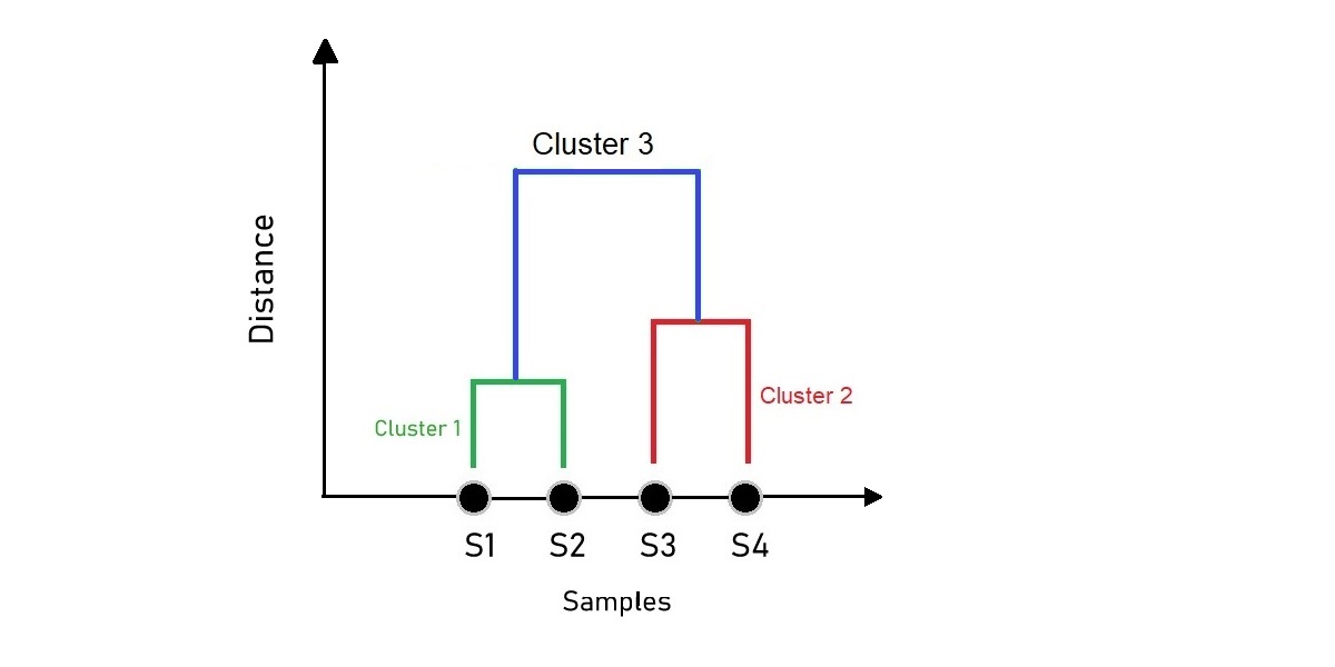
The figure we get is what we call a Dendrogram. A dendrogram is a tree-like diagram that illustrates the arrangement of the clusters produced by the corresponding analyses. The samples on the x-axis are arranged automatically representing points with close proximity that will stay closer to each other.
Choosing the optimal number of clusters can be a tricky task. But as a rule of thumb, we look for the clusters with the longest “branches” or the “longest dendrogram distance”. The optimal number of clusters is also subjected to expert knowledge, context, etc.
With enough idea in mind, let’s proceed to implement one in python.
Hierarchical clustering with Python
Let’s dive into one example to best demonstrate Hierarchical clustering
We’ll be using the Iris dataset to perform clustering. you can get more details about the iris dataset here.
1. Plotting and creating Clusters
sklearn.cluster module provides us with AgglomerativeClustering class to perform clustering on the dataset.
As an input argument, it requires a number of clusters (n_clusters), affinity which corresponds to the type of distance metric to use while creating clusters, linkage linkage{“ward”, “complete”, “average”, “single”}, default=”ward”.
The linkage criterion determines which distance to use between the given sets of observations.
You can know more about AgglomerativeClustering class here.
#Importing required libraries

from sklearn.datasets import load_iris
from sklearn.cluster import AgglomerativeClustering
import numpy as np
import matplotlib.pyplot as plt


#Getting the data ready

data = load_iris()
df = data.data
#Selecting certain features based on which clustering is done
df = df[:,1:3]


#Creating the model

agg_clustering = AgglomerativeClustering(n_clusters = 3, affinity = 'euclidean', linkage = 'ward')

#predicting the labels

labels = agg_clustering.fit_predict(df)

#Plotting the results

plt.figure(figsize = (8,5))
plt.scatter(df[labels == 0 , 0] , df[labels == 0 , 1] , c = 'red')
plt.scatter(df[labels == 1 , 0] , df[labels == 1 , 1] , c = 'blue')
plt.scatter(df[labels == 2 , 0] , df[labels == 2 , 1] , c = 'green')
plt.show()

In the above code, we considered the number of clusters to be 3.
This was evident as the iris dataset contains only 3 distinct classes but in real-life scenarios, we perform unsupervised clustering on data because we have no information about the label that each data point belongs to.
Hence finding out the optimal number of clusters is subjected to some domain expertise. But there are few methods available to find out optimal clusters that we’ll talk about in a future article.
2. Plotting Dendrogram
The scipy.cluster module contains the hierarchy class which we’ll make use of to plot Dendrogram.
The hierarchy class contains the dendrogram method and the linkage method.
The linkage method takes the dataset and the method to minimize distances as parameters i.e. ward and returns a linkage matrix which when provided to dendrogram method creates Dendrogram of the fitted data.
Let’s see what the above statement means by an example.
#Importing libraries
from sklearn.datasets import load_iris
from sklearn.cluster import AgglomerativeClustering
import numpy as np
import matplotlib.pyplot as plt
from scipy.cluster.hierarchy import dendrogram , linkage

#Getting the data ready

data = load_iris()
df = data.data
#Selecting certain features based on which clustering is done
df = df[:,1:3]

#Linkage Matrix
Z = linkage(df, method = 'ward')

#plotting dendrogram
dendro = dendrogram(Z)
plt.title('Dendrogram')
plt.ylabel('Euclidean distance')
plt.show()

Conclusion
In this article, we tried to get some basic intuition behind what Hierarchical clustering really is and its working mechanism. We also got some idea about how a dendrogram gets constructed and finally implemented HC in Python.
Happy Learning!


