🚀 Supercharge your YouTube channel's growth with AI.
Try YTGrowAI FreeLinear Regression from Scratch in Python

In this article, we’ll learn to implement Linear regression from scratch using Python. Linear regression is a basic and most commonly used type of predictive analysis.
It is used to predict the value of a variable based on the value of another variable. The variable we want to predict is called the dependent variable.
The variable we are using to predict the dependent variable’s value is called the independent variable.
The simplest form of the regression equation with one dependent and one independent variable.
y = m * x + b
where,
- y = estimated dependent value.
- b = constant or bias.
- m = regression coefficient or slope.
- x = value of the independent variable.
Linear Regression from Scratch
In this article, we will implement the Linear Regression from scratch using only Numpy.
1. Understanding Loss Function
While there are many loss functions to implement, We will use the Mean Squared Error function as our loss function.

A mean squared error function as the name suggests is the mean of squared sum of difference between true and predicted value.
As the predicted value of y depends on the slope and constant, hence our goal is to find the values for slope and constant that minimize the loss function or in other words, minimize the difference between y predicted and true values.
2. Optimization Algorithm
Optimization algorithms are used to find the optimal set of parameters given a training dataset that minimizes the loss function, in our case we need to find the optimal value of slope (m) and constant (b).
One such Algorithm is Gradient Descent.
Gradient descent is by far the most popular optimization algorithm used in machine learning.
Using gradient descent we iteratively calculate the gradients of the loss function with respect to the parameters and keep on updating the parameters till we reach the local minima.
3. Steps to Implement Gradient Descent
Let’s understand how the gradient descent algorithm works behind the scenes.
Step-1 Initializing the parameters
Here, we need to initialize the values for our parameters. Let’s keep slope = 0 and constant = 0.
We will also need a learning rate to determine the step size at each iteration while moving toward a minimum value of our loss function.
Step -2 Calculate the Partial Derivatives with respect to parameters
Here we partially differentiate our loss function with respect to the parameters we have.

Step – 3 Updating the parameters
Now, we update the values of our parameters using the equations given below:

The updated values for our parameters will be the values with which, each step minimizes our loss function and reduces the difference between the true and predicted values.
Repeat the process to reach a point of local minima.
4. Implementing Linear Regression from Scratch in Python
Now that we have an idea about how Linear regression can be implemented using Gradient descent, let’s code it in Python.
We will define LinearRegression class with two methods .fit( ) and .predict( )
#Import required modules
import numpy as np

#Defining the class
class LinearRegression:
    def __init__(self, x , y):
        self.data = x
        self.label = y
        self.m = 0
        self.b = 0
        self.n = len(x)

    def fit(self , epochs , lr):

        #Implementing Gradient Descent
        for i in range(epochs):
            y_pred = self.m * self.data + self.b

            #Calculating derivatives w.r.t Parameters
            D_m = (-2/self.n)*sum(self.data * (self.label - y_pred))
            D_b = (-1/self.n)*sum(self.label-y_pred)

            #Updating Parameters
            self.m = self.m - lr * D_m
            self.c = self.b - lr * D_c

    def predict(self , inp):
        y_pred = self.m * inp + self.b
        return y_pred
We create an instance of our LinearRegression class with training data as the input to the class and initialize the bias and constant values as 0.
The .fit( ) method in our class implements Gradient Descent where with each iteration we calculate the partial derivatives of the function with respect to parameters and then update the parameters using the learning rate and the gradient value.
With the .predict( ) method we are simply evaluating the function y = m * x + b , using the optimal values of our parameters, in other words, this method estimates the line of best fit.
4. Testing the Linear Regression Model
Now as we created our class let’s test in on the data. Learn more about how to split training and testing data sets. You can find the datasets and other resources used within this tutorial here.
#importing Matplotlib for plotting
import matplotlib.pyplot as plt

#Loding the data
df = pd.read_csv('data_LinearRegression.csv')

#Preparing the data
x = np.array(df.iloc[:,0])
y = np.array(df.iloc[:,1])

#Creating the class object
regressor = LinearRegression(x,y)

#Training the model with .fit method
regressor.fit(1000 , 0.0001) # epochs-1000 , learning_rate - 0.0001

#Prediciting the values
y_pred = regressor.predict(x)

#Plotting the results
plt.figure(figsize = (10,6))
plt.scatter(x,y , color = 'green')
plt.plot(x , y_pred , color = 'k' , lw = 3)
plt.xlabel('x' , size = 20)
plt.ylabel('y', size = 20)
plt.show()
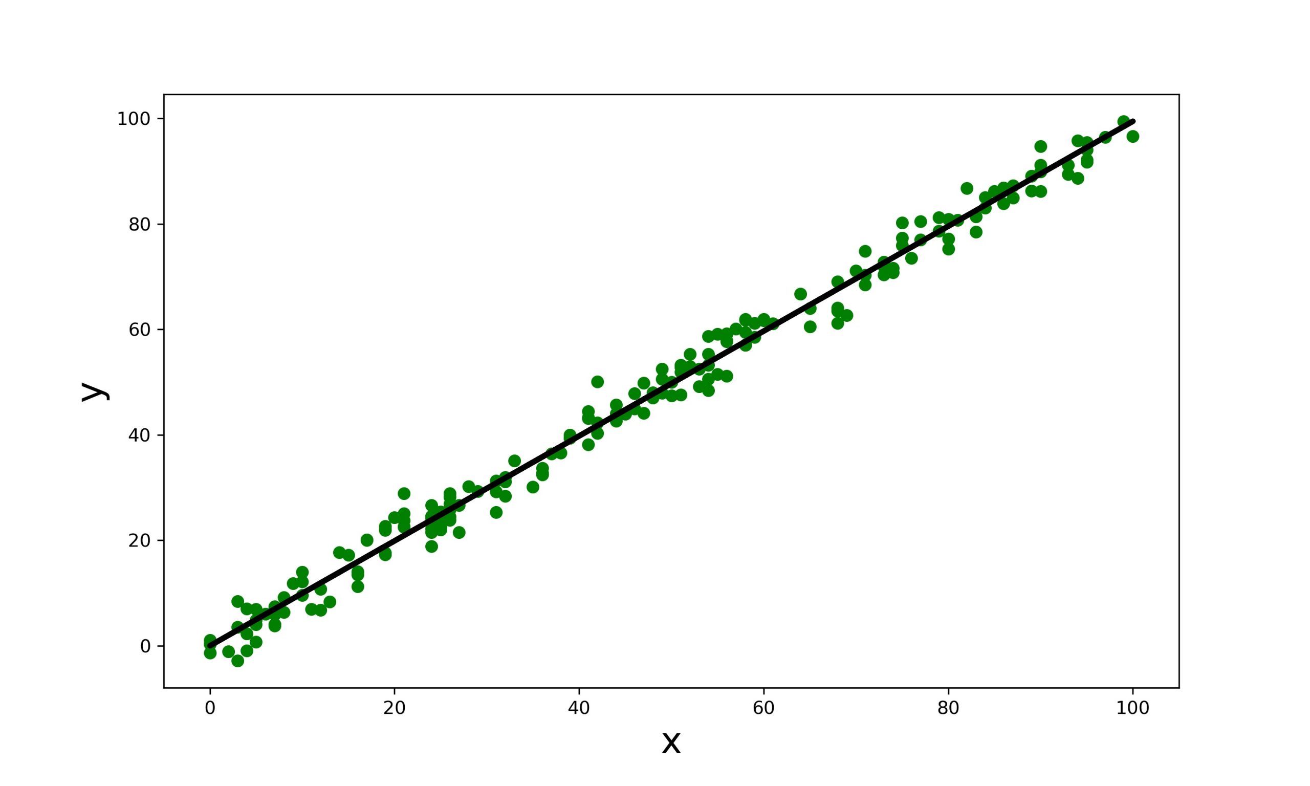
Works fine !
Conclusion
This article was all about how we can make a Linear Regression model from scratch using only Numpy. The goal of this tutorial was to give you a deeper sense of what Linear Regression actually is and how it works.
Till we meet next time.
Happy Learning!


