🚀 Supercharge your YouTube channel's growth with AI.
Try YTGrowAI FreeNaive Bayes Classifier with Python

Naïve Bayes Classifier is a probabilistic classifier and is based on Bayes Theorem.
In Machine learning, a classification problem represents the selection of the Best Hypothesis given the data.
Given a new data point, we try to classify which class label this new data instance belongs to. The prior knowledge about the past data helps us in classifying the new data point.
The Naive Bayes Theorem
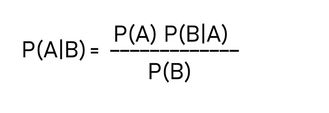
Bayes theorem gives us the probability of Event A to happen given that event B has occurred. For example.
What is the probability that it will rain given that its cloudy weather? The probability of rain can be called as our hypothesis and the event representing cloudy weather can be called as evidence.
- P(A|B) – is called as a posterior probability
- P(B|A) – is the conditional probability of B given A.
- P(A) – is called as Prior probability of event A.
- P(B) – regardless of the hypothesis, it is the probability of event B to occur.
Now that we have some idea about the Bayes theorem, let’s see how Naive Bayes works.
How Does the Naïve Bayes Classifier Work?
To demonstrate how the Naïve Bayes classifier works, we will consider an Email Spam Classification problem which classifies whether an Email is a SPAM or NOT.
Let’s consider we have total 12 emails. 8 of which are NOT-SPAM and remaining 4 are SPAM.
- Number of NOT-SPAM emails – 8
- Number of SPAM emails – 4
- Total Emails – 12
- Therefore, P(NOT-SPAM) = 8/12 = 0.666 , P(SPAM) = 4/12 = 0.333
Suppose the entire Corpus comprises just four words [Friend, Offer, Money, Wonderful]. The following histogram represents the word count of each word in each category.

We’ll now calculate the conditional probabilities of each word.
The formula given below will calculate the Probability of the word Friend to occur given the mail is NOT-SPAM.

Calculating the probabilities for the whole text corpus.

Now that we have all the prior and conditional Probabilities, we can apply the Bayes theorem to it.
Suppose we get an Email: “Offer Money” and based on our previously calculated probabilities we need to classify it as SPAM or NOT-SPAM.

The Probability of Email to be a SPAM given the words Offer and Money is greater than the Probability of the mail to be NOT-SPAM. (0.0532 > 0.00424).
Hence our Classifier will classify this Email to be a SPAM. In summary, we just calculated the posterior Probability as shown in the Bayes theorem.
If we came across a variable that is not present in the other categories then the word count of that variable becomes 0 (zero) and we will be unable to make a prediction.
This Problem is also known as a “Zero Frequency” problem. To avoid this, we make use of smoothening methods. i.e. Laplace estimation. Smoothening techniques do not affect the conditional probabilities.
Types of Naïve Bayes Classifier:
- Multinomial – It is used for Discrete Counts. The one we described in the example above is an example of Multinomial Type Naïve Bayes.
- Gaussian – This type of Naïve Bayes classifier assumes the data to follow a Normal Distribution.
- Bernoulli – This type of Classifier is useful when our feature vectors are Binary.
Implementing Naïve Bayes with Python
We’ll make use of the breast cancer Wisconsin dataset. You can know more about the dataset here.
Scikit Learn provides us with GaussianNB class to implement Naive Bayes Algorithm.
#Loading the Dataset
from sklearn.datasets import load_breast_cancer

data_loaded = load_breast_cancer()
X = data_loaded.data
y = data_loaded.target
The dataset has 30 features using which prediction needs to be done. We can access the data just by using .data method. The dataset has features and target variables.
#Splitting the dataset into training and testing variables
from sklearn.model_selection import train_test_split

X_train, X_test, y_train, y_test = train_test_split(data.data, data.target, test_size=0.2,random_state=20)

#keeping 80% as training data and 20% as testing data.
Now, importing the Gaussian Naive Bayes Class and fitting the training data to it.
from sklearn.naive_bayes import GaussianNB

#Calling the Class
naive_bayes = GaussianNB()

#Fitting the data to the classifier
naive_bayes.fit(X_train , y_train)

#Predict on test data
y_predicted = naive_bayes.predict(X_test)
The .fit method of GaussianNB class requires the feature data (X_train) and the target variables as input arguments(y_train).
Now, let’s find how accurate our model was using accuracy metrics.
#Import metrics class from sklearn
from sklearn import metrics

metrics.accuracy_score(y_predicted , y_test)
Accuracy = 0.956140350877193
We got accuracy around 95.61 %
Feel free to experiment with the code. You can apply various transformations to the data prior to fitting the algorithm.
Conclusion
In this article, we got some intuition about the Naive Bayes classifier. We have also seen how to implement Naive Bayes using sklearn. Happy Learnning!


