🚀 Supercharge your YouTube channel's growth with AI.
Try YTGrowAI FreeWhat is SciPy? Complete Beginner’s Guide to Scientific Python

Scientific calculations in Python, such as estimating an integral or finding a minimum, lead you to SciPy. It’s a free library of numerical algorithms that works on the arrays NumPy provides.
I’ll map SciPy’s subpackages to the calculations they handle, and show how SciPy relates to NumPy.
What is SciPy?
SciPy is a free, open-source Python library of numerical algorithms for scientific computing. A numerical algorithm calculates an answer from numbers, such as estimating an integral or finding where a function reaches a minimum.
NumPy supplies the multidimensional arrays that SciPy builds on, so the libraries work together in the same program. You might prepare measurements in a NumPy array, then pass them to a SciPy statistical routine.
| Library | Its job | When to reach for it |
|---|---|---|
| NumPy | Arrays and numerical array operations | Create an array or calculate its average |
| SciPy | Scientific algorithms and specialized numerical structures | Estimate an integral or solve an optimization problem |
| pandas | Labeled Series and DataFrame objects | Organize measurements by column and row labels |
The difference between NumPy and SciPy depends on the calculation, because their capabilities overlap in areas such as linear algebra. Use the function whose documented options fit your problem rather than treating SciPy as a replacement for NumPy.
The SciPy user guide organizes its numerical algorithms by scientific domain. SciPy calculates numerical results rather than rearranging equations into symbolic formulas. The project is distributed under the BSD license.
Which SciPy subpackage fits your calculation?
A subpackage groups related functions under a name such as scipy.integrate. Importing from that group keeps the algorithm’s purpose visible without loading every name into your program.
- Choose the mathematical task before choosing a function.
- Read the function’s input requirements and returned values.
- Keep NumPy imports separate when you also need array operations.
Optimization and integration both accept a Python function in these examples, but one searches for a minimum while the other estimates area under a curve.
| Subpackage | Calculation | Input to think about |
|---|---|---|
| scipy.optimize | Find a minimum or solve an equation | An objective function and suitable search conditions |
| scipy.integrate | Estimate a definite integral | A function and integration limits |
| scipy.stats | Evaluate distributions or statistical tests | Sample data and the test’s assumptions |
| scipy.linalg | Solve linear systems and related matrix problems | Coefficient arrays with compatible shapes |
| scipy.signal | Filter or analyze sampled signals | Samples and the meaning of their sampling rate |
| scipy.interpolate | Estimate values between known observations | Known coordinates and measured values |
SciPy also provides sparse arrays for data with numerous zero entries and spatial structures for tasks involving coordinates. The subpackage reference gives you the wider module map when your calculation falls outside this table.
Try SciPy in a project environment
To run the calculations, use Python with SciPy installed in the environment that executes your script. You need to recognize a Python function and its return value, but the examples introduce their mathematical assumptions as they use them.
I installed SciPy in a fresh environment with Python 3.14.7, and pip installed NumPy as its dependency. The executed examples used SciPy 1.18.1 with NumPy 2.5.3.
python -m pip install scipy
Using python -m pip ties the install to the interpreter named by python. Activate your project environment first, and use that same interpreter when starting the script or selecting a notebook kernel.
python -c 'import scipy, numpy; print(scipy.__version__); print(numpy.__version__)'
The command printed 1.18.1 followed by 2.5.3 in the example environment. It proves those packages import in that interpreter, not in every Python installation on the computer.
The official installation instructions describe project-based tools as well as environment-based installs. For platform-specific steps, use the AskPython SciPy installation tutorial.
How SciPy searches for a function’s minimum
Optimization searches for an input that makes an objective function’s value smaller. An objective function is the quantity you want to minimize, so you must define what a lower value means before asking a solver to find it.
For example, (x – 4) ** 2 + 3 reaches its minimum when x is 4 because the squared term then becomes zero. I chose minimize_scalar() with the bounded method because this function has one input and the search interval is known.
from scipy.optimize import minimize_scalar

result = minimize_scalar(
    lambda x: (x - 4) ** 2 + 3,
    bounds=(0, 10),
    method="bounded",
)
print(f"Minimum: x={result.x:.3f}, f(x)={result.fun:.3f}")
print(f"Success: {result.success}")
print(f"Message: {result.message}")
The lambda supplies the function SciPy evaluates at candidate inputs, while bounds limits its search to the interval from 0 to 10. The solver returns an OptimizeResult object, which carries the answer together with information about how the search ended.
Save this example as optimization_demo.py. For a virtual environment named env in the project directory, run the file with its interpreter.
./env/bin/python optimization_demo.py
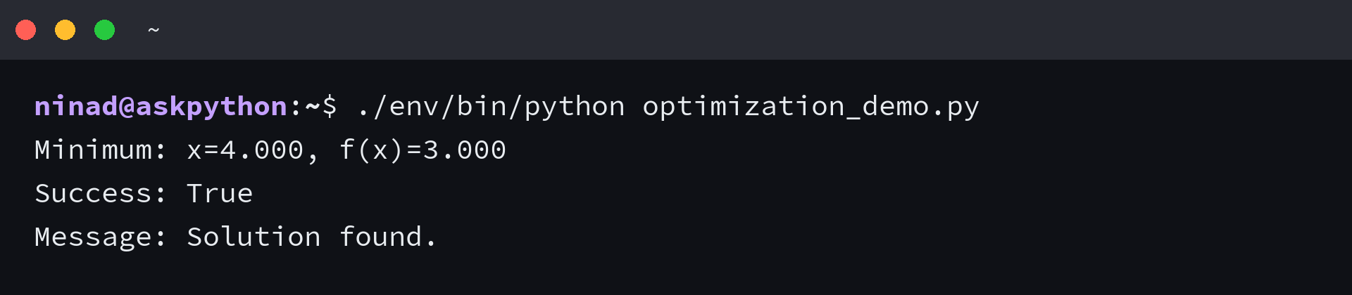
The result separates x=4.000, the input location, from f(x)=3.000, the function value there. Success is True and the message is Solution found., so the solver reports successful termination for this calculation.
I ran the same function with bounds from 6 to 10 and got x=6.000 with f(x)=7.000, again with success=True. The search succeeded even though those bounds excluded the function’s minimum at 4.
The minimize_scalar() documentation describes its methods as local minimizers, so a success flag cannot establish a global minimum for an arbitrary function. For multiple variables or constraints, compare the methods in the SciPy minimize tutorial.
Read the integral and statistical results
Numerical integration estimates the accumulated value of a function over an interval. For x squared from 0 to 1, the exact area is one third, which makes this a calculation you can check independently of SciPy.
quad() takes a callable and the interval’s limits, then returns both an integral estimate and an estimate of its absolute error. Unpack the pair into separate variables so the uncertainty remains visible beside the answer.
from scipy.integrate import quad

area, error = quad(lambda x: x**2, 0, 1)
print(f"Area: {area:.6f}")
print(f"Estimated absolute error: {error:.2e}")
The calculation returned 0.333333 with an estimated absolute error of 3.70e-15. That estimate concerns the numerical integration. It does not account for an incorrect formula or inaccurate measurements used to construct it.
The quad() reference requires a convergent integral for valid results. If you have sampled observations rather than a function you can evaluate between points, choose a method for sampled data instead of assuming quad() accepts the same input.
Compare independent samples with Welch’s test
A hypothesis test measures how compatible your observations are with a stated statistical assumption. Here the null hypothesis is that the populations behind two independent samples have equal means, and Welch’s test allows their variances to differ.
Passing equal_var=False selects Welch’s test instead of the equal-variance test that ttest_ind() uses by default. The groups are illustrative data, not measurements from an experiment.
from scipy import stats

group_a = [10, 12, 13, 11, 14]
group_b = [15, 16, 14, 18, 17]
result = stats.ttest_ind(group_a, group_b, equal_var=False)
print(f"statistic={result.statistic:.3f}, p-value={result.pvalue:.4f}")
I used equal_var=False and got a statistic of -4.000 with a p-value of 0.0039. The negative statistic reflects the first group’s lower mean, while the p-value describes how extreme this result is under the equal-means hypothesis and the test’s assumptions.
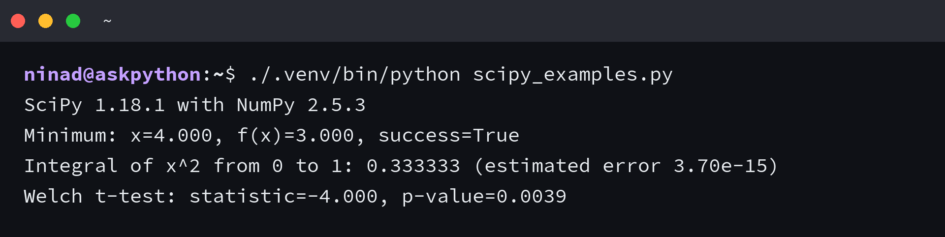
A p-value is not the probability that the null hypothesis is true, and it does not measure whether an effect is useful. Independent observations and a defensible sampling process still matter even when the function executes without an error.
| Returned value | What it tells you | What it cannot establish |
|---|---|---|
| quad() area | Numerical estimate of the specified integral | Whether your formula describes the intended system |
| quad() error | Estimated absolute numerical error | Total uncertainty in your model or measurements |
| ttest_ind() p-value | Tail probability under the null hypothesis | Probability that the null hypothesis is true |
For integration details, continue with the worked quad() guide. The SciPy statistics guide describes tests and distributions. The ttest_ind() reference explains its statistical options and returned fields.
Why an import or numerical result can mislead
An import failure concerns the environment before it concerns the mathematics. A returned number needs a different investigation, because the algorithm can finish successfully while answering a question defined by unsuitable inputs.
| Symptom | Check before changing the calculation |
|---|---|
| ModuleNotFoundError for scipy | Use the interpreter where SciPy was installed, including the matching notebook kernel |
| Failed building wheel for scipy | Compare your Python and platform with the official installation options and available binary distributions |
| Unexpected minimum with success=True | Inspect bounds and the solver’s local search assumptions |
| Integration warnings or implausible area | Check convergence and whether the integrand has discontinuities |
| A small p-value treated as proof | Examine sample independence and the interpretation of the null hypothesis |
NumPy and SciPy functions belong to separate namespaces, so import NumPy explicitly for NumPy operations. Treat a question about similar function names as a reason to compare their current documentation, not as evidence that the entire namespaces are interchangeable.
Excluding 4 from the interval changed the reported minimum, while the success flag remained True because the solver met its stopping conditions.
Change the bounds before trusting the answer
Try the quadratic with bounds from 6 to 10, where the function is increasing throughout the allowed interval. The solver approaches the lower boundary rather than the minimum at 4, so its rounded output becomes x=6.000 and f(x)=7.000.
from scipy.optimize import minimize_scalar

result = minimize_scalar(
    lambda x: (x - 4) ** 2 + 3,
    bounds=(6, 10),
    method="bounded",
)
print(f"Minimum: x={result.x:.3f}, f(x)={result.fun:.3f}")
print(f"Success: {result.success}")
Success remains True in this experiment. Use a calculation with an independently known answer when learning a SciPy routine. You can then distinguish understanding the returned object from trusting the problem you supplied.
SciPy questions beyond the first calculation
Choosing between libraries also raises questions about dependencies and performance. Those choices depend on the operation you need rather than the package name alone.
Does installing SciPy also install NumPy?
SciPy depends on NumPy, so pip installs a compatible NumPy dependency when it is needed. Import NumPy separately when your program calls NumPy functions.
Is SciPy faster than NumPy?
There is no blanket speed ranking between the libraries. Compare the specific algorithm on your data and installed numerical libraries before drawing a performance conclusion.
Is SciPy the same as pandas?
SciPy provides numerical algorithms, while pandas provides labeled table structures. You can organize observations in pandas and use SciPy for a calculation on the numeric data.